
Q: What does the B. in Benoit B. Mandelbrot stand for?
A: Benoit B. Mandelbrot
Benoit B Mandelbrot (1924-2010) is best known for his work on fractals (in fact, he is credited with coining the term fractal) and in particular the Mandelbrot set which he started investigating in 1979. The name was given to it by a later mathematician, Douady, in tribute to him. People have written entire books about the Mandelbrot set to there is no way to do justice to all aspects of it in a single post. Instead, I will concentrate only on one aspect of it, using it to illustrate the difference between deterministic and predictable.
What is the Mandelbrot Set?
The Mandelbrot set is defined by a very simple looking equation:
![]()
Don’t let the apparent simplicity fool you however. This is a recurrence relation, defining a sequence of numbers. It tells you if you know one number in a sequence what to do to get the next one. For example, if the constant c=1 and we initially start with z0=0, then the sequence is 0,1,2,5,26, and so on getting bigger and bigger. However, if c=-1 and we again initially start with z0=0, then the sequence is 0,-1,0,-1,0,-1, and so on, forever oscillating between 0 and -1, thus remaining bounded.
However let us now think of z as a complex number. This means that z contains a real and an imaginary part, and we could write it as z=x+iy. Similarly, the constant c is a complex number, which we will write as c=cx+icy. The recurrence relation then tells us if we have a complex number z, or equivalently two coordinates x and y (which can be thought of as a point on the plane) how to get to the next complex number, or equivalently the next point on the plane. We could then either leave it in the dangerously simple looking form above, or write out explicitly the equations for the coordinates, which are

We will always consider starting at the origin, x0=0, y0=0, and think about how the trajectory changes as we vary the constants cx and cy.
As we can think of this as the evolution of coordinates on a plane, we can plot the trajectory as points, starting at the origin and proceeding as the set of points for n=1,2,3, and so on. Below, I’ve done this for three different values of the constants cx and cy. In blue, (cx,cy) = (0.4,0.4); in red, (cx,cy) = (-0.7,0.25); and in green (cx,cy) = (-0.3,-0.7).
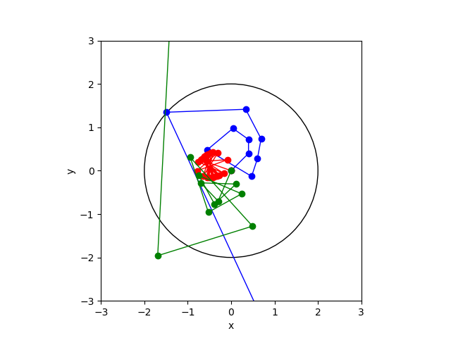
These trajectories look somewhat chaotic – we are beginning to see explicitly that the simplicity of our equation defining the trajectory does not mean the resulting trajectory will be simple! But these trajectories are complexly deterministic. If I tell you the coordinates of the constant c, you could easily work out as many steps of the trajectory as you wish, at least in principle (a computer helps though!) I will demonstrate shortly however that the key words here are in principle – despite the apparent simplicity of the equations, it is actually not so easy to evolve to follow the trajectory for many points in the future (even with a good computer). But before getting to that, let us finish defining the Mandelbrot set.
As trainee (either by doing or desire) scientists, we are used to specific quantitative questions – such as where will the moon by in 10 days time, or 100 days time, or 1000 days time, or so on. Or in the case of the Mandelbrot recurrence relation, you could ask for given constants (cx,cy), what will be the coordinates after 100 iterations, or 1000, or so on. But let us ask instead a more general question, not about specifics of the solution (we can already see above that the trajectories look a bit crazy) but about the general nature of it. Specifically, you will see that I have drawn a circle in the figure above of radius 2 centred on the origin. This is because the question I will ask is:
For given constants (cx,cy), does the trajectory stay within the black circle or not?
It obviously starts in the circle, as is starts at the origin, but what happens after that? In the examples above, we can see that the red trajectory does stay within the circle (at least as far as we have drawn it, but it turns out it will always stay inside), while the blue and green trajectories go outside the circle. If the trajectory does stay within the circle, then the point (cx,cy) is part of the Mandelbrot set. If the trajectory goes outside the circle, then the point (cx,cy) is not part of the Mandelbrot set.
The more common definition given is that the point (cx,cy) is part of the Mandelbrot set if the resulting trajectory is bounded (i.e. doesn’t scupper off to infinity in some direction), but one can show (supposing one is Mandelbrot that is) that the alternative definition in terms of the circle above is equivalent to this. An analogy with the moon would be instead of asking where the moon is in 1000 days, we merely ask if the moon will still be orbiting the earth in 1000 days (answer: yes, but extend that to several billion years and the answer is less clear).
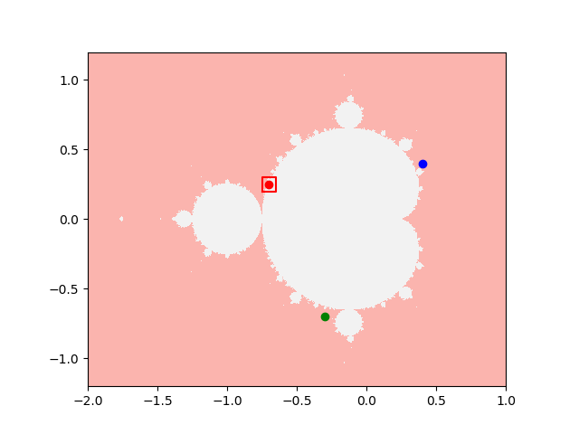
So the Mandelbrot set is the set of all points (cx,cy) where the trajectory stays within the circle. What does this look like? It’s plotted in the figure below. The axes are cx and cy, and the white bit is the Mandelbrot set. In other words, choose your value of cx and cy,, look at the graph below; if it is white, then the trajectories stay inside the circle, if it is pink, they don’t. I’ve also plotted the position of the three examples used in the previous plot – where as you can see, the blue and green points are not in the Mandelbrot set (they lie on the pink bit), while the red point is in the Mandelbrot set (the white bit).

This image is already beginning to show complex emergent behaviour, that you wouldn’t have expected from such a simple equation. You can find far more beautiful plots online, where different colourings correspond to different behaviours within the set, or how many iterations it takes to leave the circle outside the set, or many other things. One can talk about the facial nature of the set, the self-similarity, or more complicated things such as is the set simply connected (a technical maths thing that is important to mathematicians but nobody has been able to show whether the Mandelbrot set has this property or not – its an open question to this day).
Let me not get too much off track and return to the main thread of this post.
Deterministic but not predictable
I’ve plotted the Mandelbrot set, so as well as being a deterministic equation, surely then the behaviour is predictable? Not so fast.
Lets as an example focus on the red point. And let us suppose that we are physicists so we know we can only measure the value of the point with finite accuracy. Or alternatively, we are mathematicians working out the evolution on a computer, with an imperfect computer that represents the values of cx and cy to finite accuracy (as for example, all computers outside of sci-fi do).
To demonstrate this, notice I’ve drawn a little red box around the red point – so let us suppose this is the limits on how accurately we know the values of cx and cy. Below, I’ve zoomed into the graph above – the plot below corresponds to exactly the red square in the plot above.
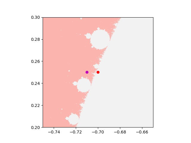
Notice that if I really did only have this accuracy, I might be anywhere in the plot above, so a roughly 50% chance of my trajectory remaining in the circle, and a 50% chance of it not. So we’ve accepted that the equation governing the evolution is completely deterministic, and in this case, looks really simple, However, incomplete knowledge of the value of the parameter (and in the real world, all knowledge is incomplete – nothing is known to infinite accuracy) means not only can we not predict the location of the point many iterations into the future, we are reduced to probabilities to predicts the nature of the solution. And you can also see above that this isn’t just because I gave a large uncertainty to cx and cy. You can see that were I to draw a little box around the red point again and zoom in, I’d get a picture looking rather similar. And so on.
We can demonstrate this further by plotting a few trajectories again – the red spot is exactly where it always was, but the magenta spot is moved to the left by only 0.01 units. The trajectories for the red point that we saw at the very beginning is replotted below, with the trajectory for the purple point added.
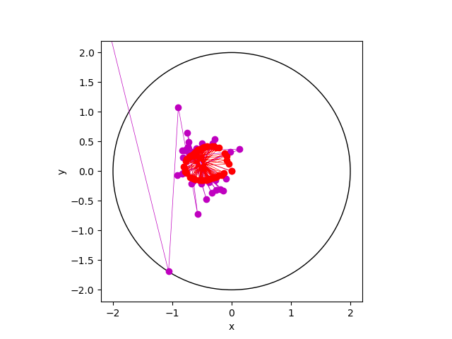
The thing to notice here is not just that the trajectories start to diverge after a number of iterations, but that they look like they have nothing to do with each other. This is what is referred to in the biz as extreme sensitivity to initial conditions.
The take home message
There are a few points worth making here as a postscript. Firstly, I know of no physical system described (or approximated) by the Mandelbrot recurrence relation. However, there are many problems in physics with similar properties, such as the double pendulum, or Poincare’s three body problem of orbital dynamics. In these cases, the base equations look more complicated, although by fact of being to write them make the system deterministic. When one puts them on a computer, the computer doesn’t care if the set of equations put in is `deceptively simple’ or not – but conceptually from a pedagogic point of view, it is nice to have a simple model illustrating the desired behaviour, which is why I chose the example of the Mandelbrot set. The general concepts are universal, even if the model itself is only interesting from an abstract point of view.
Secondly, it is worth directly contrasting the behaviour seen here with a non-chaotic system, such as two bodies interacting via gravity. In this case, there are two possible behaviours: the two bodies orbit each other, or they don’t – i.e. one body first approaches the other, gets to a point of least distance, then goes past getting further away, never to approach again. If two bodies start in orbit, then they will continue in orbit forever; if they don’t start in orbit, they will `scatter’ off each other never to approach again. This is in contrast to the three-body problem, where e.g. the moon may orbit the earth orbiting the sun for a long period of time, but one cannot say for sure that this behaviour will last forever. Or in the case of the Mandelbrot set where the trajectory may bounce around inside the circle for many iterations before deciding to leave.
Finally, I’d like to mention that it is not just the presence of a boundary of the Mandelbrot set that makes the behaviour unpredictable/chaotic. Anything with a phase transition or bifurcation will have values of the parameter close to the phase boundary where a small uncertainty could tip it over the edge. For example, a topical example would be simple models in epidemiology where we know there is a ‘reproduction rate’ r, telling us how many people on average each person infects. And in these models, there is a bifurcation at r=1. If r>1, the number of infected people grows; if r<1 it decreases. If r>1, there is an epidemic, if r<1, there isn’t. Suppose r is close to 1. We may have some uncertainty so we don’t know if it is above or below 1, and obviously there is a very different result in these two cases. However, as time evolves, as soon as the two trajectories differ by enough to distinguish them, we would see if the infections are increasing or decreasing, and infer the nature of the solution. Contrast that with the situation in the picture above, where the red and purple trajectories diverge for short times but stay within the same little cluster, which has a size of about 1 unit in each direction – far bigger than the initial difference between parameters. If I’d stopped the computer simulation after fewer iterations, you would have seen that the red and magenta trajectories indeed diverge from each other – but you wouldn’t ever have predicted that the magenta one would at some point escape the circle, while the red one wouldn’t.
So it is not just the presence of a phase boundary that gives us this unpredictability – that alone would typically be called a tipping point – which you’ve most likely heard about in discussions about climate change. There, the uncertainty may tell you are close enough to the bifurcation point that you don’t know which way you’ll go. But that is quite a different story. Here, we also have a phase boundary which is itself an extremely complex object – a fractal. This is what makes it different.
And all of this from the simple looking quadratic equation at the top. Forget what your teacher at school told you. Quadratic equations are cool!
Hi Great article can I ask could the border of the shape be defined as the sum of an infinite series, and hence a formula for the area is possible maybe?