Public policy on insurance risk classification is typically perceived as a trade-off between two types of argument. On the one hand, social arguments against discrimination suggest a need for limits on insurers’ ability to use individual data in setting premiums. On the other hand, economic arguments under the rubric of ‘adverse selection’ or ‘anti-selection’ suggest that such limits make insurance markets work less well.
Our main point is that this trade-off is often illusory. Not all adverse selection is adverse, and public policy should not seek to eliminate all adverse selection. Limits on insurance discrimination that induce the right amount of adverse selection (but not too much adverse selection) can lead to more risk being transferred, and more losses being compensated. This makes insurance work better for society as a whole.
To fix ideas, it helps to think of a specific market, say life insurance. The point can then be illustrated by the following toy example.
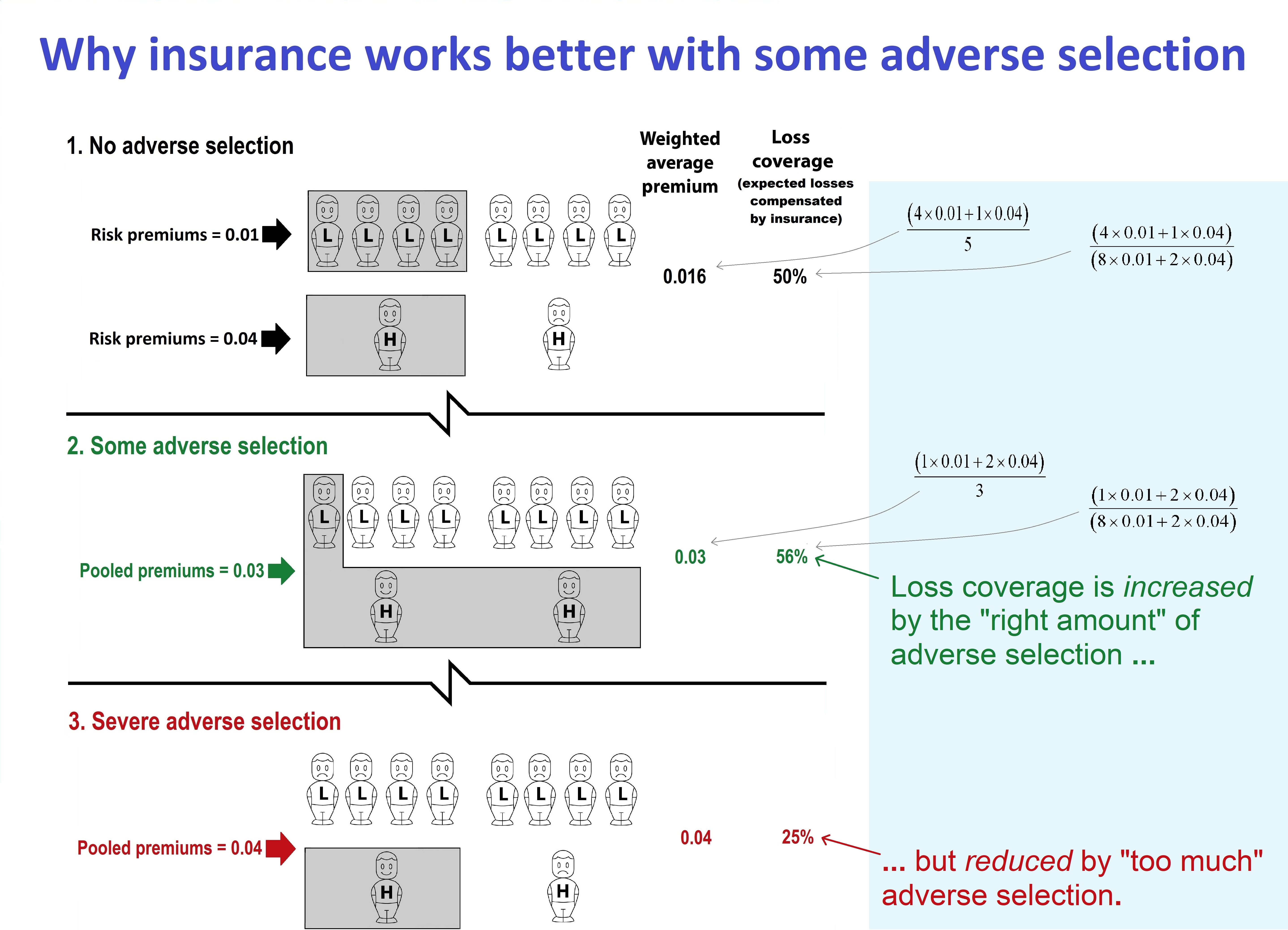
Consider a population of just ten people, comprising two risk-groups: eight low risks with probability of loss 0.01, and two high risks with probability of loss 0.04. Assume that all losses and insurance cover are for unit amounts (this simplifies the presentation, but it is not necessary). Then, consider three alternative scenarios for insurance risk classification.
In Scenario 1, members of each risk-group are charged a price equal to their true probability of loss. The responses of high and low risks are the same: exactly half the members of each risk-group decide to buy. The shading denotes the people who are covered.
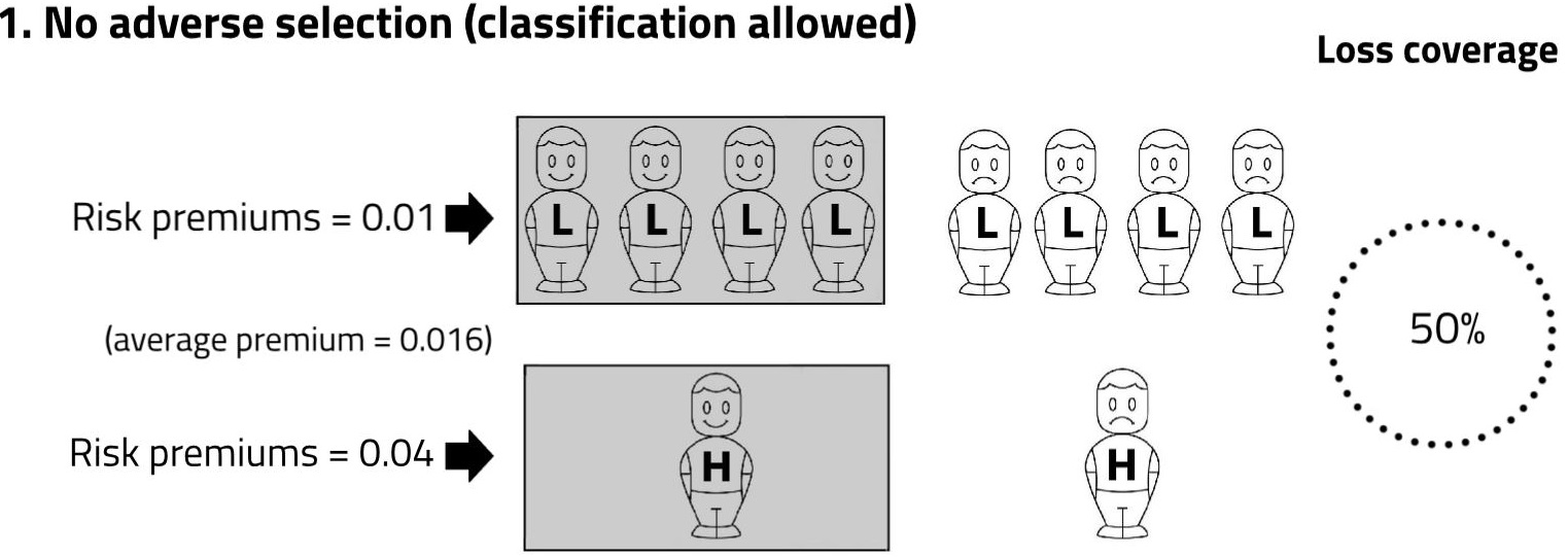
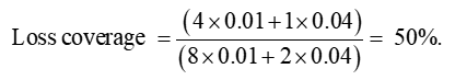
The average premium paid in Scenario 1 is 0.016. Exactly half the population’s expected losses are compensated by insurance. We describe this as ‘loss coverage’ of 50%. The calculation is expected insured losses, divided by expected population losses, that is:
Next, consider Scenario 2. Risk classification has now been banned, so insurers have to charge a common pooled premium to everyone, somewhere in between the two previous premiums. At the pooled premium, high risks are more likely to buy, and low risks less likely (adverse selection). The shading denotes the three people who are now covered. The pooled premium is 0.03, which is set so that expected profits on low risks exactly offset expected losses on high risks.
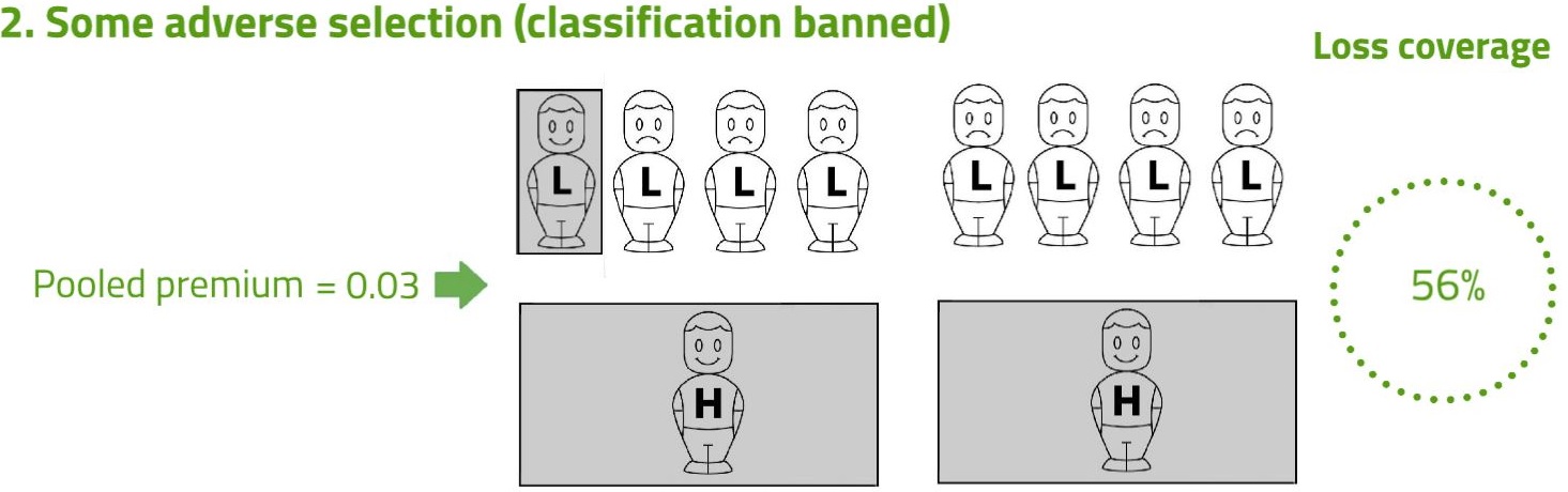
Note that in Scenario 2, the average premium paid is higher (0.03 compared with 0.016 before), and the number of people covered is lower (three compared with five before). These are the essential features of adverse selection, which the example fully represents. But there is a surprise: despite the adverse selection, Scenario 2 achieves a higher transfer of risk, and hence a higher expected compensation of losses.
Intuitively, this can be seen by comparing the shaded areas. In Scenario 1, the shading over one high risk has the same area as the shading over four low risks. Those equal areas represent equal quantities of risk transferred. Then notice that in Scenario 2, the total shaded area is larger than in Scenario 1. This represents more risk being transferred, and hence more expected losses being compensated.
The visual intuition is confirmed when we calculate the loss coverage:
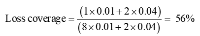
which is higher than the 50% in Scenario 1.
Scenario 2, with a higher expected fraction of the population’s losses compensated by insurance –higher loss coverage – seems superior from a social viewpoint to Scenario 1. The superiority of Scenario 2 arises not despite adverse selection, but because of adverse selection.
So from society’s viewpoint, some adverse selection is a good thing. But like most good things, it’s not good without limit. If adverse selection goes too far, this can lead to lower loss coverage. Scenario 3 illustrates this case.
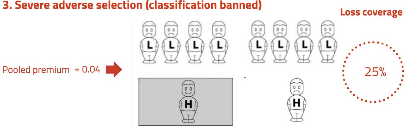
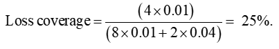
The one low-risk purchaser in Scenario 2 has now dropped out of the market (further adverse selection), so the break-even premium has risen to 0.04. The response of the high risks to this premium is the same as in Scenario 1: exactly half (i.e. one) of them buys insurance. The shaded area is smaller than in both the earlier scenarios. The loss coverage is:
Taken together, the three scenarios suggest that risk classification increases loss coverage if it induces the ‘right amount’ of adverse selection (Scenario 2), but reduces loss coverage if it induces ‘too much’ adverse selection (Scenario 3). Which of Scenario 2 or Scenario 3 actually prevails depends on the response of high and low risks to changes in prices – that is, the ‘demand elasticities’ of high and low risks.
The arithmetic illustrated by the toy example applies broadly. It does not depend on the specific context of life insurance, or on any unusual choice of numbers for the example. When we incorporate features which the example omits for simplicity, such as profit and expense loadings, this does not change the basic point.
From a social viewpoint, compensation of the population’s losses is the main purpose of insurance. Policymakers may therefore prefer risk classification regimes that maximise loss coverage. This typically means regimes that produce a non-zero level of adverse selection, and somewhat lower numbers insured than if adverse selection were eliminated.
Our argument contrasts with orthodox economic arguments that policymakers should either seek to minimise adverse selection, or make a trade-off against other policy preferences such as dislike of discrimination. The orthodox arguments highlight that adverse selection leads to a rise in average price, and fall in numbers insured. What these arguments miss is that adverse selection also leads to a shift in coverage towards higher risks – from a social viewpoint, the ‘right’ risks, those who need insurance most. If this shift in coverage is large enough, it can more than outweigh the fall in numbers insured. So in aggregate, loss coverage is increased.
An economist might suggest that rather than maximising loss coverage, policymakers should seek to maximise “social welfare”, defined as expected utility for a randomly selected member of the population. But utility is a figment of economists’ imagination, never directly observable (like phlogiston in 18th-century chemistry!). And it is hard to measure utility: if we infer it from willingness-to-pay, it may be contaminated by cognitive errors, inattention, inertia and probability neglect. The advantage of loss coverage, for public policy purposes, is that it is observable, and therefore measurable.
In practice. a complete ban on risk classification is unlikely; that is an exaggerated feature of the toy example. But the logic of the example does suggest that to maximise loss coverage, policymakers need to set limits on insurers’ use of data. Using too much data to classify risk too finely and remove all adverse selection reduces the quantum of voluntary risk transfer, and so makes insurance work less well.
Finally, note that the concept of loss coverage is not predicated on any special consideration for the high risks. It targets the compensation of losses in general, with no preference for losses arising from any particular group. It is a measure of the overall efficacy of insurance in effecting voluntary transfer of risk. It is a matter of insurance arithmetic, not of ethics.
Further reading: Book, academic papers, other articles.
In one summary picture: