The latest version of the paper can be found on arxiv:
eDNAPlus: A unifying modelling framework for DNA-based biodiversity monitoring
The model uses as input the reads for each species, i.e. the count data indicating the number of times the DNA of each species has been read at a given PCR for a given sample.
It is a hierarchical model, which accounts for variation, error and noise in the three levels of metabarcoding surveys
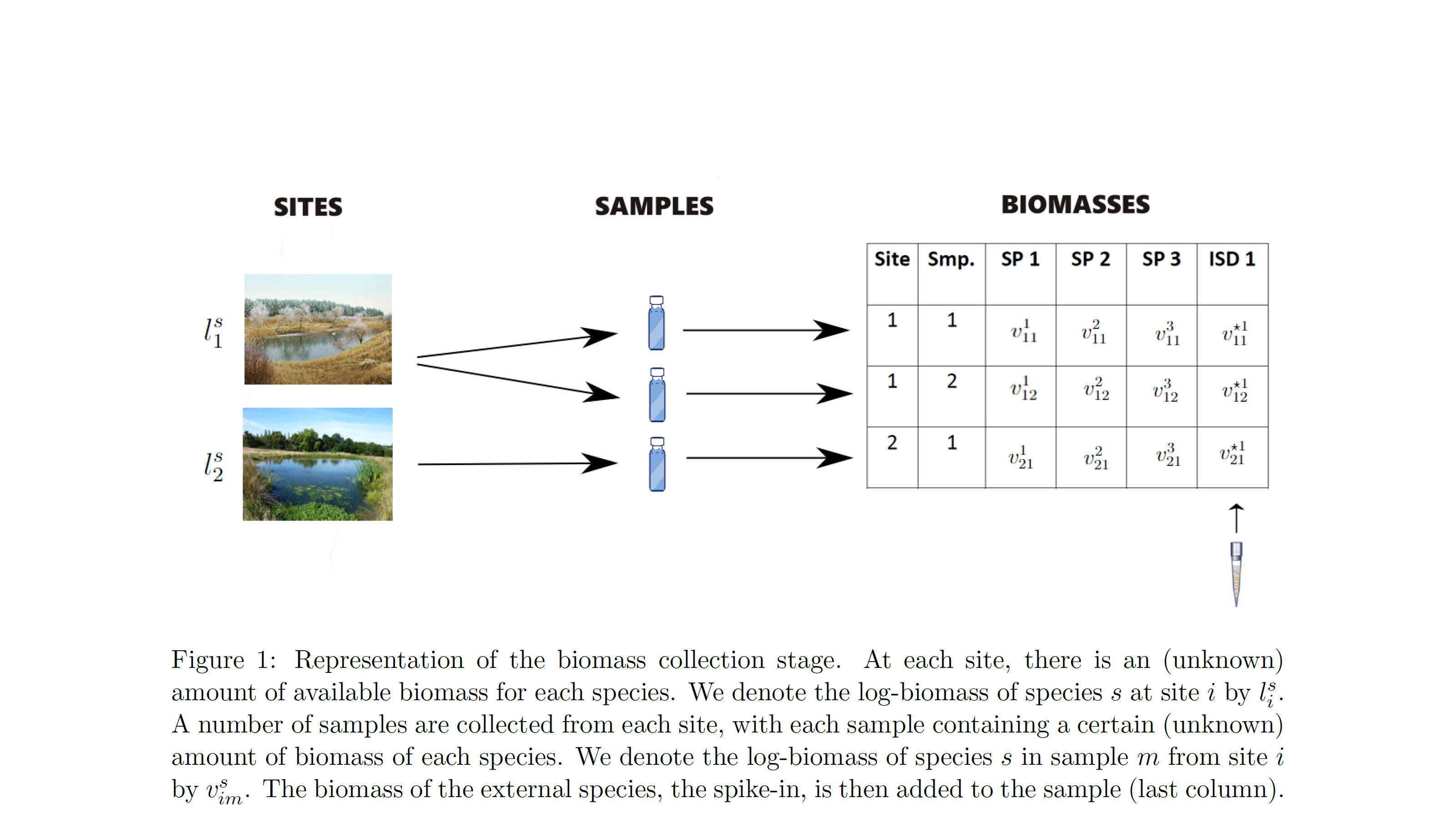
- biomass availability: the amount of biomass for each species available for collection at each surveyed site
- biomass collection: the amount of biomass for each species collected in each physical sample from each surveyed site
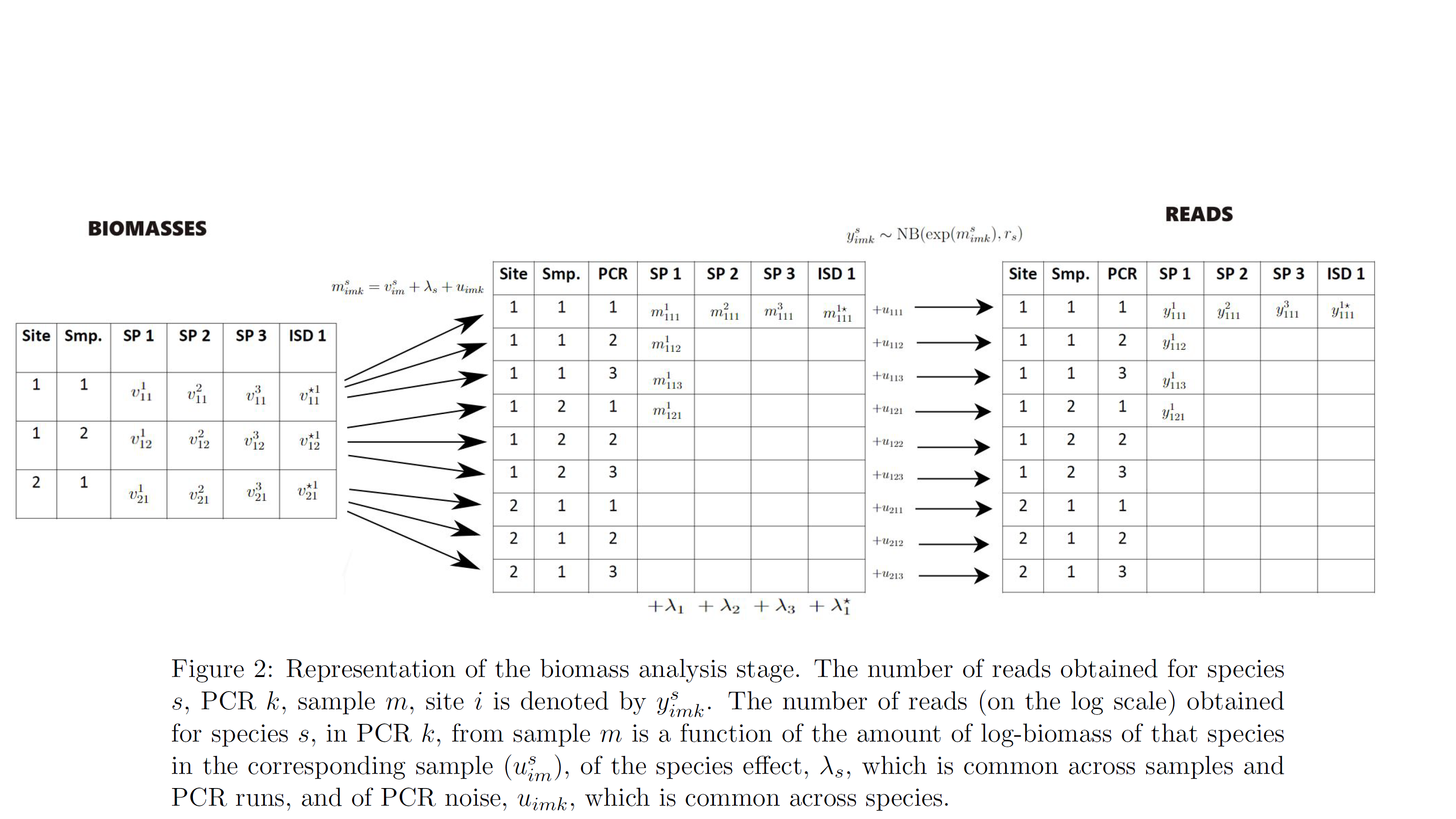
- biomass analysis: the amount of biomass detected for each species and physical sample at each PCR run.
Data are only available from the biomass analysis stage, i.e. the reads, whereas the other two stages are unobservable (latent). Each of the above stages is modelled using regression-type models that include both fixed effects and random effects.
At the biomass availability stage, the model accounts for variation between sites due to their observable differences, eg landscape characteristics and due to species correlations, eg species that tend to co-occur (fixed effects). It also accounts for random noise between sites, ie. for the fact that identical sites in terms of their characteristics (fixed effects) can have different amounts of biomass of each species due to chance (random effects).
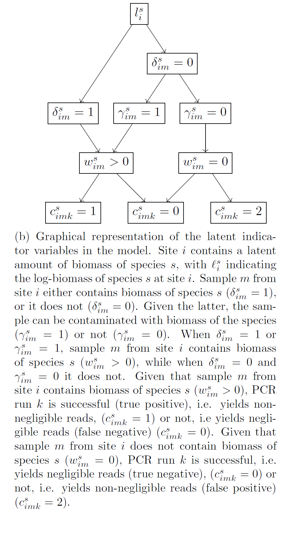
At the biomass collection stage, the model accounts for variation between samples due to their observable differences, eg “size” in terms of litres of water or amount of soil or number of leeches, and due to species effects, i.e. for the fact that our sample collection approach will be more effective for collecting biomass of some species over others (fixed effects). It also accounts for random noise between samples, ie. for the fact that identical samples in terms of their characteristics (fixed effects) can have different amounts of biomass of each species due to chance (random effects). Finally, it accounts for error, namely it estimates the probability that we fail to collect biomass of a species in a sample and for the probability that the collected biomass in a sample is the result of contamination.
At the biomass analysis stage, the model accounts for species effects, i.e. for the fact that our PCR (eg primers) approach will be more effective for reading the biomass of some species over others (fixed effects). It also accounts for random noise between PCRs, ie. for the fact that identical PCRs in terms of their characteristics (fixed effects) can give different reads for each species due to chance (random effects). Finally, it accounts for error, namely it estimates the probability that a PCR fails to give non-negligible reads for a species that had non-negligible biomass in the sample (i.e. the PCR should have given “large” reads for a species but it did not, false negative error) and for the probability that a PCR gives non-negligible reads for a species that had negligible amount of biomass in the sample (the PCR should not have given “large” reads for a species but it did, false positive error).
The model also accounts for spike-ins i.e. the process during which a known amount of biomass of an external species is added to the collected biomass. This process is helpful for understanding the level of PCR noise.